Thoughts

Mind melting calculations to solve a shape sorting conundrum 18th February 2019

We promised you a behind the scenes look at the challenges we faced when dealing with a shape sorting problem when exploring how custom development breaks new ground.

This article isn't called mind melting without good reason...

This article is for the mathematically minded reader who enjoys exploring the formulas, models and calculations that we used to solve this complex problem.

But first to recap..

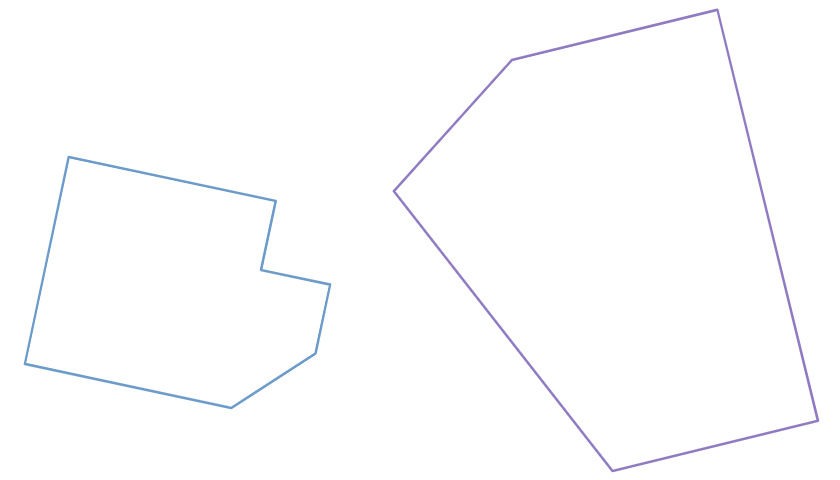
Our property sales client asked us to create an automated feature to determine whether a builder's plan fits within a developer's lot. Sounds simple, except the shapes were polygons and were able to be rotated, translated or reflected to achieve a match, which made this request much more unique.

Research

Our process always begins with research to see if there are any available implementations to springboard from, (which there weren't) but we did find a research paper that addressed our requirements.

The Polygon Containment Problem, (Chazelle, 1983, 1-33) described mathematical proofs for various types of polygon containment. In our specifications, the lot (P) and Plan (Q) may or may not have been convex polygons, so Chazelle's "naive approach" was used.

From this proof, we were able to construct an algorithm that runs in O[p^3q^3(p+q)log(p+q)] time. Still a hefty process to be running, but much better than any brute force attempt. The proof was the theoretical backing behind our solution, but was vague on the steps that needed to be taken to implement it. The calculations involved and converting the algorithm from on paper into clear, concise, maintainable code was a challenge, but one that we are specially equipped to tackle here a BlueSky.

The Solution

Chazelle proves that polygon containment can be found through the enumeration of stable placements between P and Q. A stable placement can be described as any placement of Q in P that results in three points of contact between the vertices of Q and the edges of P. If one vertex of Q is touching an edge of P, then Q can slide along the edge and rotate around the point of intersection without leaving the edge. This is one point of contact. If this vertex is positioned on a vertex of P, Q can rotate but not slide. If two vertices of Q are located on edges of P, then they can slide along their edges, but not rotate around any point irrespective of another. In both of these cases, two points of contact have been made. If a third point of contact is made, either one P-Q vertex contact with a P-Q edge-vertex contact or 3 P-Q edge-vertex contacts, then Q can no longer be rotated or translated without breaking contact and a stable placement has been found.

For the 3 P-Q edge-vertex contacts stable placement, chose 3 arbitrary edges or P (p1, p2, p3) and 3 arbitrary vertices of Q (Q1, Q2, Q3). The vertices from Q form a new triangle (T) whereas, with the edges from P, p1 and p2 need to intersect at some point (i.e. not be parallel). The first point of contact can be found by simply placing Q1 on p1 in any arbitrary location. The next point of contact can be found by moving Q1 to an arbitrary point within p1, such that a second vertex, Q2, touches a second edge, p2. Mathematically, this requires finding the intersection of p1 and p2, the choosing any arbitrary point on p2 that is less than the distance from Q1 to Q2 away from the intersection and placing Q2 on it.

The third stable placement is the most difficult to find. As Q1 and Q2 slide respectively up and down p1 and p2, the point Q3 traces an ellipse, centred around the intersection of p1 and p2. To find the third stable placement, the intersection between this ellipse and p3 need to be found. The angles and side lengths of Triangle Q, as well as the point of intersection of p1 and p2 can be used to find the equation of the ellipse using the method in Appendix 1. Determining the intercepts between the ellipse and p3 is described in Appendix 2.

Once a stable placement is found, the original polygon Q can be substituted for the Triangle T, using the translation and rotation transformations that were required to find the stable placement. At this point the test has been reduced to finding the polygon in polygon containment of one fixed polygon within another. Using line intersections as well as Point-in-Polygon test, we can determine whether the given placement is valid.

If the test on this placement fails, the next combination of P edges and Q vertices will need to be tested, iterating through all combinations, including the simpler possibilities where Q1 is placed on the intersection between p1 and p2. If a valid placement is still not found, reflect Q and repeat the process.

Calculations

Equation of the Q3 ellipse (Appendix 1)

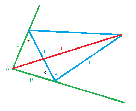
As the triangle T slides 2 vertices V1 and V2 along intersecting lines L1 and L2, the 3rd vertex of T, V3 follows an elliptical path, centred around the intersect between L1 and L2 (the origin, O). We then need to find the points of intersection between a third line L3 and the ellipse.

The distance between O and V3 is represented by the line r in figure 1. The magnitude of line r can be found through the law of cosines:

c and B are known constants, so r, p and θ are our unknown variables. Using the law of sines, we can represent p in terms of θ:

a and A are known constants, so the formula for r becomes:

This formula now represents the magnitude of r for any given angle for θ. As every r length falls on the surface of an ellipse, we can assume that all values of r fall between -π ≤ θ ≤ π.

To define the ellipse made by T3, we need to find the major axis. The major axis of an ellipse is the line that passes through the origin and the furthest point on the ellipse. The derivative of r with respect to θ will give us the rate of change of r with respect to θ. When T3 reaches its furthest point from the origin, its rate of change will dip to 0, before r starts tending back toward the origin. When dr/dθ = 0, r is at its maximum/minimum value and T3 is intersecting with one of the axes of the ellipse.

The chain and product rules are used to find the derivative of r^2

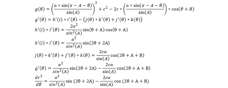
To find a root of r, we need to set the rate of change of r with respect to θ to 0:

The value for θ cannot be isolated and solved simply, so must be found through approximation. The Newton-Raphson technique can be used to quickly find a root of the function. For this, we need the second derivative:

Now we can iterate through the Newton-Raphson method until we have a root of dr^2/dθ:

The initial value can be an arbitrary location between -π and π. Each new x value should bring the result of f(x) closer to zero. When it is within a given tolerance (e.g. ±0.00001) then the θ value can be used as an approximation of a root. There should be 2 roots between (-π/2 <= θ <= π/2), one being the maximum, and another being the minimum. The roots of an ellipse should be separated by π/2. Sub the roots of θ back into the original equation to and compare the two to determine the maximum and minimum r values.

The original x and y axes should be rotated to make the x-axis parallel with the major axis of the ellipse. If the x-axis is currently parallel to p, then the angle of rotation can be found using the law of sines:

All points in the system need to be modified by the rotational matrix:

Now that the x-axis is parallel to the major-axis of the ellipse and values are known for the max and min r values, the equation of the ellipse can be determined:

Intersection of the Q3 ellipse and p3 (Appendix 2)

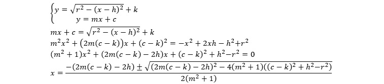
We can now use this equation to find the intersections between the ellipse and any line (L3) in the form of y=mx+c. Note, if the line is in the form y=c or x=d then the quadratic formula is not necessary, being able to be subbed directly into the equation of the ellipse.

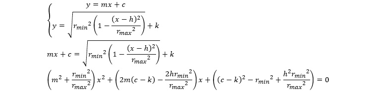
As this is now a quadratic equation, we can use the quadratic formula to solve for the roots:

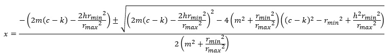
If

then the solution will be complex, meaning that the line does not intercept the ellipse at any point. If

then no roots exist and the line does not intercept with the ellipse at any point (real or imaginary).

Each of the intersections (P1 and P2) between the ellipse and L3 represent a possible stable placement between the two polygons. To test whether the point is a match, place V3 on P and rotate the triangle until V1 and V2 fall on lines L1 and L2 respectively. There will only be one rotation angle that allows all three pairs in the combination to be made. To find the angle that the triangle needs to be rotated from its original position, first, create a circle for V1 and V2 around P and find the intercept between each circle and their respective line. There will be 0-2 intercepts.

The quadratic formula can now be used to find the roots. Iterate through the combinations of intercepts and use the one that results in the distance apart being exactly the length of side a.

A triangle can then be formed between V3, V2 and the intercept corresponding to V2 with L2. The angle at V3 will be the angle the triangle needs to rotate to place the triangle in the stable placement position. Lastly, we can now translate the test polygon to place V3 on the test P, rotating it by the angle found above.

Once the polygon is stably placed, a regular, "Polygon in Polygon" algorithm can be run to check whether the transformed polygon is wholly contained within the stationary polygon (all points are within the polygon found through rays, no edges intersect between the two polygons). This process must then be repeated on all combinations of 3 edges of the stationary polygon with three vertices of the transformable polygon.

References

Chazelle, Bernard. 1983. "The Polygon Containment Problem." Advances in Computing Research 1 (1): 1-33.

Ben Hewitt

5 years ago

Systems programming Custom Solutions

Recent thoughts